42 how to show labels in excel chart
How to Show Percentage in Pie Chart in Excel? - GeeksforGeeks Jun 29, 2021 · It can be observed that the pie chart contains the value in the labels but our aim is to show the data labels in terms of percentage. Show percentage in a pie chart: The steps are as follows : Select the pie chart. Right-click on it. A pop-down menu will appear. Click on the Format Data Labels option. The Format Data Labels dialog box will appear. Where is labels in excel? - scottick.firesidegrillandbar.com How do I show percentage data labels in Excel? Right click the pie chart again and select Format Data Labels from the right-clicking menu. 4. In the opening Format Data Labels pane, check the Percentage box and uncheck the Value box in the Label Options section.
Excel tutorial: How to customize axis labels Instead you'll need to open up the Select Data window. Here you'll see the horizontal axis labels listed on the right. Click the edit button to access the label range. It's not obvious, but you can type arbitrary labels separated with commas in this field. So I can just enter A through F. When I click OK, the chart is updated.
How to show labels in excel chart
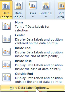
How to Add Labels to Show Totals in Stacked Column Charts in Excel In the chart, right-click the "Total" series and then, on the shortcut menu, select Add Data Labels. 9. Next, select the labels and then, in the Format Data Labels pane, under Label Options, set the Label Position to Above. 10. While the labels are still selected set their font to Bold. 11. how to add data labels into Excel graphs - storytelling with data 10 Feb 2021 — Right-click on a point and choose Add Data Label. You can choose any point to add a label—I'm strategically choosing the endpoint because that's ... Excel tutorial: How to use data labels Generally, the easiest way to show data labels to use the chart elements menu. When you check the box, you'll see data labels appear in the chart. If you have more than one data series, you can select a series first, then turn on data labels for that series only. You can even select a single bar, and show just one data label.
How to show labels in excel chart. Unable to see the Label Position in excel chart. Additionally, I found a workaround for it. You can set the position of a label first, then click Label Options > Data Label Series > Clone Current Label to quickly apply custom data label formatting to the other data points in the series. Best regards, Jazlyn. -----------. How To Add Axis Labels In Excel [Step-By-Step Tutorial] First off, you have to click the chart and click the plus (+) icon on the upper-right side. Then, check the tickbox for 'Axis Titles'. If you would only like to add a title/label for one axis (horizontal or vertical), click the right arrow beside 'Axis Titles' and select which axis you would like to add a title/label. Editing the Axis Titles Custom data labels in a chart - Get Digital Help 21 Jan 2020 — Press with right mouse button on on any data series displayed in the chart. · Press with mouse on "Add Data Labels". · Press with mouse on Add ... Excel charts: add title, customize chart axis, legend and data labels To show data labels inside text bubbles, click Data Callout. How to change data displayed on labels To change what is displayed on the data labels in your chart, click the Chart Elements button > Data Labels > More options… This will bring up the Format Data Labels pane on the right of your worksheet.
How to Place Labels Directly Through Your Line Graph in Microsoft Excel Right-click on top of one of those circular data points. You'll see a pop-up window. Click on Add Data Labels. Your unformatted labels will appear to the right of each data point: Click just once on any of those data labels. You'll see little squares around each data point. Then, right-click on any of those data labels. You'll see a pop-up menu. How to use data labels in a chart - YouTube Excel charts have a flexible system to display values called "data labels". Data labels are a classic example a "simple" Excel feature with a huge range of o... Learn How to Show or Hide Chart Axes in Excel - Lifewire Select Chart Elements, the plus sign ( + ), to open the Chart Elements menu. To hide all axes, clear the Axes check box. To hide one or more axes, hover over Axes to display a right arrow. Select the arrow to display a list of axes that can be displayed or hidden on the chart. Clear the check box for the axes you want to hide. Add or remove data labels in a chart - support.microsoft.com Click Label Options and under Label Contains, select the Values From Cells checkbox. When the Data Label Range dialog box appears, go back to the spreadsheet and select the range for which you want the cell values to display as data labels. When you do that, the selected range will appear in the Data Label Range dialog box. Then click OK.
How to add or move data labels in Excel chart? - ExtendOffice In Excel 2013 or 2016. 1. Click the chart to show the Chart Elements button . 2. Then click the Chart Elements, and check Data Labels, then you can click the arrow to choose an option about the data labels in the sub menu. See screenshot: In Excel 2010 or 2007. 1. click on the chart to show the Layout tab in the Chart Tools group. See ... Add a DATA LABEL to ONE POINT on a chart in Excel Steps shown in the video above: Click on the chart line to add the data point to. All the data points will be highlighted. Click again on the single point that you want to add a data label to. Right-click and select ' Add data label ' This is the key step! Right-click again on the data point itself (not the label) and select ' Format data label '. Custom Chart Data Labels In Excel With Formulas Follow the steps below to create the custom data labels. Select the chart label you want to change. In the formula-bar hit = (equals), select the cell reference containing your chart label's data. In this case, the first label is in cell E2. Finally, repeat for all your chart laebls. How to Insert Axis Labels In An Excel Chart | Excelchat We will go to Chart Design and select Add Chart Element Figure 6 - Insert axis labels in Excel In the drop-down menu, we will click on Axis Titles, and subsequently, select Primary vertical Figure 7 - Edit vertical axis labels in Excel Now, we can enter the name we want for the primary vertical axis label.
Creating a chart with dynamic labels - Microsoft Excel 2016
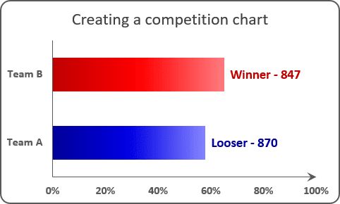
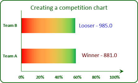
Text Labels on a Horizontal Bar Chart in Excel - Peltier Tech Dec 21, 2010 · In this tutorial I’ll show how to use a combination bar-column chart, in which the bars show the survey results and the columns provide the text labels for the horizontal axis. The steps are essentially the same in Excel 2007 and in Excel 2003. I’ll show the charts from Excel 2007, and the different dialogs for both where applicable.
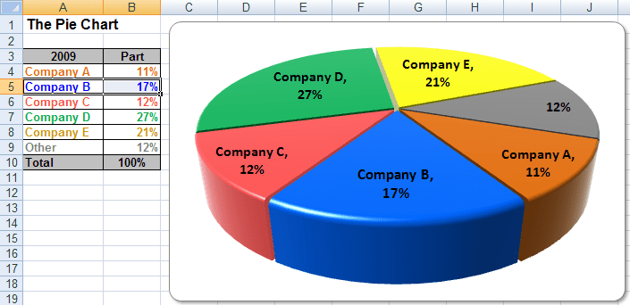
Excel 3-D Pie Charts
Create Excel Waterfall Chart Template - Download Free Template Jun 09, 2022 · Right-click on the chart and select Change Chart Type; change chart type of Before and After Series to Line. Click either of the Before or After Series Lines, click the green plus button on the top right corner of the waterfall chart and check the box for Up/Down Bars. The Up-Bars show positive changes, while the Down-Bars show negative changes.
Excel: Formatting Charts in Excel 2010 with Layout - Excel Articles
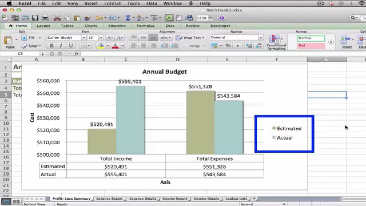
Excel charts: how to move data labels to legend - Microsoft Tech Community You can't do that, but you can show a data table below the chart instead of data labels: Click anywhere on the chart. On the Design tab of the ribbon (under Chart Tools), in the Chart Layouts group, click Add Chart Element > Data Table > With Legend Keys (or No Legend Keys if you prefer)

Bubble Chart: How to create it in excel - DataWitzz
Dynamically Label Excel Chart Series Lines - My Online Training Hub Step 1: Duplicate the Series. The first trick here is that we have 2 series for each region; one for the line and one for the label, as you can see in the table below: Select columns B:J and insert a line chart (do not include column A). To modify the axis so the Year and Month labels are nested; right-click the chart > Select Data > Edit the ...
Position Chart Legend & Display Gridlines in Microsoft Excel: MOOC - YouTube
Excel Charts: Dynamic Label positioning of line series - XelPlus Select your chart and go to the Format tab, click on the drop-down menu at the upper left-hand portion and select Series "Budget". Go to Layout tab, select Data Labels > Right. Right mouse click on the data label displayed on the chart. Select Format Data Labels. Under the Label Options, show the Series Name and untick the Value.

Excel 2010 Tutorial Changing Chart Labels Microsoft Training Lesson 21.3 - YouTube
How To Create Labels In Excel - nudelsorten.info Select mailings > write & insert fields > update labels. In the next dialog box, select the sheet in excel that contains the list. Select mailings > write & insert fields > update labels. The create cards dialog window will appear: Now you need to tell word which fields you want and in what order.
Creating a chart with dynamic labels - Microsoft Excel 2013
Excel Chart not showing SOME X-axis labels - Super User Apr 05, 2017 · In Excel 2013, select the bar graph or line chart whose axis you're trying to fix. Right click on the chart, select "Format Chart Area..." from the pop up menu. A sidebar will appear on the right side of the screen. On the sidebar, click on "CHART OPTIONS" and select "Horizontal (Category) Axis" from the drop down menu.

31 What Is A Label In Excel - Labels For Your Ideas
charts - Excel, giving data labels to only the top/bottom X% values ... Here is what you can do, in stages: 1) Create a data set next to your original series column with only the values you want labels for (again, this can be formula driven to only select the top / bottom n values). See column D below. 2) Add this data series to the chart and show the data labels. 3) Set the line color to No Line, so that it does ...
Excel Charts: Positive/Negative Axis Labels on a Bar Chart
How to display text labels in the X-axis of scatter chart in ... Display text labels in X-axis of scatter chart. Actually, there is no way that can display text labels in the X-axis of scatter chart in Excel, but we can create a line chart and make it look like a scatter chart. 1. Select the data you use, and click Insert > Insert Line & Area Chart > Line with Markers to select a line chart. See screenshot:
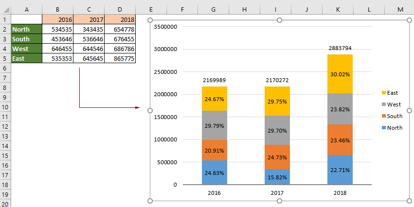
How to show percentages in stacked column chart in Excel?
How to add data labels from different column in an Excel chart? 18 Nov 2021 — How to add data labels from different column in an Excel chart? · 1. Right click the data series in the chart, and select Add Data Labels > Add ...

Excel Chart Elements: Parts of Charts in Excel | ExcelDemy
How to Use Cell Values for Excel Chart Labels How to Use Cell Values for Excel Chart Labels Make your chart labels in Microsoft Excel dynamic by linking them to cell values. When the data changes, the chart labels automatically update. In this article, we explore how to make both your chart title and the chart data labels dynamic.
Displaying Numbers in Thousands in a Chart in Microsoft Excel
Edit titles or data labels in a chart - support.microsoft.com On a chart, click the label that you want to link to a corresponding worksheet cell. On the worksheet, click in the formula bar, and then type an equal sign (=). Select the worksheet cell that contains the data or text that you want to display in your chart. You can also type the reference to the worksheet cell in the formula bar.

Line Chart in Excel - Easy Excel Tutorial
How to Add Total Data Labels to the Excel Stacked Bar Chart Apr 03, 2013 · For stacked bar charts, Excel 2010 allows you to add data labels only to the individual components of the stacked bar chart. The basic chart function does not allow you to add a total data label that accounts for the sum of the individual components. Fortunately, creating these labels manually is a fairly simply process.
Excel Charts: Creating Custom Data Labels - YouTube
Chart Labels | MrExcel Message Board 29 minutes ago. #1. I have a chart that has 2 series (Budget - The green column & Spend - The blue column) where I want to hide labels where there is a zero value. I also need to show the label to 1 decimal place of the unit type (thousands) but where I have applied the number format of '#""' to the Spend column, it shows with no decimal places.

10 Tips for Making Charts in Excel | Mekko Graphics
How to Add Data Labels in Excel - Excelchat | Excelchat After inserting a chart in Excel 2010 and earlier versions we need to do the followings to add data labels to the chart; Click inside the chart area to display the Chart Tools. Figure 2. Chart Tools. Click on Layout tab of the Chart Tools. In Labels group, click on Data Labels and select the position to add labels to the chart.
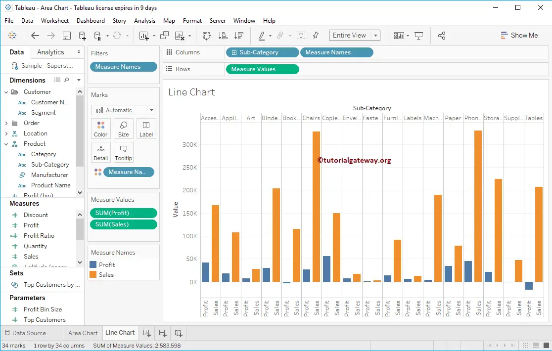
Grouped Bar Chart in Tableau
How to Create a Bar Chart With Labels Above Bars in Excel In the Format Data Labels pane, under Label Options selected, set the Label Position to Inside Base. 10. Then, under Label Contains, check the Category Name option and uncheck the Value and Show Leader Lines options. 11. Next, while the labels are still selected, click on Text Options, and then click on the Textbox icon. 12.
Custom Chart Labels Using Excel 2013 | MyExcelOnline
How to Add Labels to Scatterplot Points in Excel - Statology Next, click anywhere on the chart until a green plus (+) sign appears in the top right corner. Then click Data Labels, then click More Options… In the Format Data Labels window that appears on the right of the screen, uncheck the box next to Y Value and check the box next to Value From Cells.
Post a Comment for "42 how to show labels in excel chart"