42 how to show data labels as percentage in excel

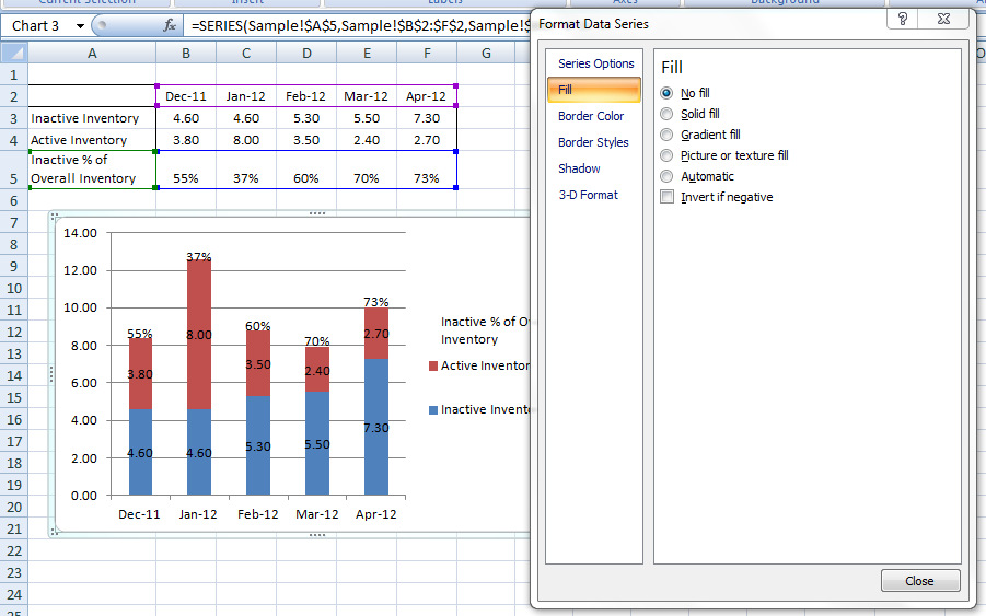
Add or remove data labels in a chart - support.microsoft.com Tip: You can use either method to enter percentages — manually if you know what they are, or by linking to percentages on the worksheet.Percentages are not calculated in the chart, but you can calculate percentages on the worksheet by using the equation amount / total = percentage.For example, if you calculate 10 / 100 = 0.1, and then format 0.1 as a percentage, the number will … Stacked bar charts showing percentages (excel) - Microsoft Community What you have to do is - select the data range of your raw data and plot the stacked Column Chart and then add data labels. When you add data labels, Excel will add the numbers as data labels. You then have to manually change each label and set a link to the respective % cell in the percentage data range.

Data Labels in Excel Pivot Chart (Detailed Analysis) Next open Format Data Labels by pressing the More options in the Data Labels. Then on the side panel, click on the Value From Cells. Next, in the dialog box, Select D5:D11, and click OK. Right after clicking OK, you will notice that there are percentage signs showing on top of the columns. 4. Changing Appearance of Pivot Chart Labels

How to show data labels as percentage in excel

DataLabels.ShowPercentage property (Excel) | Microsoft Docs This example enables the percentage value to be shown for the data labels of the first series on the first chart. This example assumes that a chart exists on the active worksheet. VB Copy Sub UsePercentage () ActiveSheet.ChartObjects (1).Activate ActiveChart.SeriesCollection (1) _ .DataLabels.ShowPercentage = True End Sub Support and feedback How to Put Count and Percentage in One Cell in Excel? Now follow the following steps to put count and percentage in one cell: Step 1: Type column header " $ Sales ( % Share)" in cell E2. Step 2: We use the Excel TEXT () function to retain excel format and the CONCAT () function to join four texts. Text 1 - Sales $ Text 2 - Open bracket Text 3 - Share % Text 4 - Close bracket How to Show Percentage in Pie Chart in Excel? - GeeksforGeeks Jun 29, 2021 · Show percentage in a pie chart: The steps are as follows : Select the pie chart. Right-click on it. A pop-down menu will appear. Click on the Format Data Labels option. The Format Data Labels dialog box will appear. In this dialog box check the “Percentage” button and uncheck the Value button. This will replace the data labels in pie chart ...

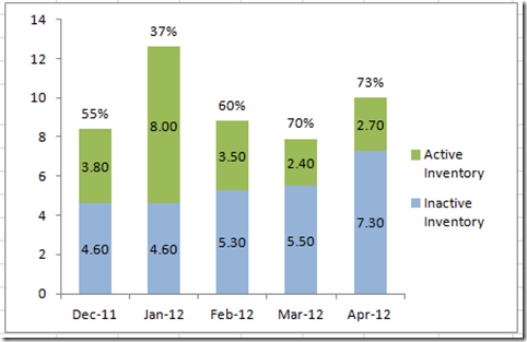
How to show data labels as percentage in excel. How to show percentages in stacked column chart in Excel? - ExtendOffice Add percentages in stacked column chart 1. Select data range you need and click Insert > Column > Stacked Column. See screenshot: 2. Click at the column and then click Design > Switch Row/Column. 3. In Excel 2007, click Layout > Data Labels > Center . In Excel 2013 or the new version, click Design > Add Chart Element > Data Labels > Center. 4. How to Display Percentage in an Excel Graph (3 Methods) Then go to the More Options via the right arrow beside the Data Labels. Select Chart on the Format Data Labels dialog box. Uncheck the Value option. Check the Value From Cells option. Then you have to select cell ranges to extract percentage values. For this purpose, create a column called Percentage using the following formula: =E5/C5 How to build a 100% stacked chart with percentages - Exceljet Now when I copy the formula throughout the table, we get the percentages we need. To add these to the chart, I need select the data labels for each series one at a time, then switch to "value from cells" under label options. Now we have a 100% stacked chart that shows the percentage breakdown in each column. How to Show Percentages in Stacked Column Chart in Excel? Dec 17, 2021 · Click Percent style (1) to convert your new table to show number with Percentage Symbol. Step 7: Select chart data labels and right-click, then choose “Format Data Labels”. Step 8: Check “Values From Cells”. Step 9: Above step popup an input box for the user to select a range of cells to display on the chart instead of default values.

Add or remove data labels in a chart - support.microsoft.com Right-click the data series or data label to display more data for, and then click Format Data Labels. Click Label Options and under Label Contains , select the Values From Cells checkbox. When the Data Label Range dialog box appears, go back to the spreadsheet and select the range for which you want the cell values to display as data labels. How to create a chart with both percentage and value in Excel? After installing Kutools for Excel, please do as this: 1. Click Kutools > Charts > Category Comparison > Stacked Chart with Percentage, see screenshot: 2. In the Stacked column chart with percentage dialog box, specify the data range, axis labels and legend series from the original data range separately, see screenshot: 3. How to Add Percentage Axis to Chart in Excel We will click on the Numbers, then choose Percentage under Category: Our Chart now looks like this: Add Percentage Axis to Chart as Secondary. The above is a fairly easy example as we had only percentages to deal with. Now we want to present all of the data we have on one chart. Luckily, newer versions of Excel are pretty helpful in this regard. How to Show Percentage Change in Excel Graph (2 Ways) May 31, 2022 · This article will illustrate how to show the percentage change in an Excel graph. Using an Excel graph can present you the relation between the data in an eye-catching way. Showing partial numbers as percentages is easy to understand while analyzing data. In the following dataset, we have a company’s Profit during the period March to September.

How to Use Excel to Make a Percentage Bar Graph | Techwalla Percentage bar graphs compare the percentage that each item contributes to an entire category. Rather than showing the data as clusters of individual bars, percentage bar graphs show a single bar with each measured item represented by a different color. Each bar on the category axis (often called the x-axis) represents 100 percent. Percentage Change Chart – Excel – Automate Excel Click on Format Data Series . 3. Change Series Overlap to 0%. 4. Change Gap Width to 0% . Your graph should look something like this so far . 5. Select Invisible Bars. 6. Click Format. 7. Select Shape Fill. 8. Click No Fill . Adding Labels. While still clicking the invisible bar, select the + Sign in the top right; Select arrow next to Data ... How to Show Percentages in Stacked Column Chart in Excel? Click Percent style (1) to convert your new table to show number with Percentage Symbol Step 7: Select chart data labels and right-click, then choose "Format Data Labels". Step 8: Check "Values From Cells". Step 9: Above step popup an input box for the user to select a range of cells to display on the chart instead of default values. Present your data in a column chart - support.microsoft.com To apply a formatting option to a specific component of a chart (such as Vertical (Value) Axis, Horizontal (Category) Axis, Chart Area, to name a few), click Format > pick a component in the Chart Elements dropdown box, click Format Selection, and make any necessary changes.Repeat the step for each component you want to modify.

10 ways to present variance analysis reports in Excel - PakAccountants.com

Data label in the graph not showing percentage option. only value ... replied to Dipil. Sep 11 2021 08:41 AM. @Dipil. You need helper columns but you don't need another chart. Add columns with percentage and use "Values from cells" option to add it as data labels. labels percent.xlsx.

How-to Put Percentage Labels on Top of a Stacked Column Chart - Excel Dashboard Templates

Excel Charts: How To Show Percentages in Stacked Charts (in ... - YouTube I also show you how you can add total values to stacks - you can also watch this video that shows that: To further improve the readability of this chart you can add the...

31 Label Pie Chart - Labels For Your Ideas

Create Dynamic Chart Data Labels with Slicers - Excel Campus Feb 10, 2016 · Typically a chart will display data labels based on the underlying source data for the chart. In Excel 2013 a new feature called “Value from Cells” was introduced. This feature allows us to specify the a range that we want to use for the labels. Since our data labels will change between a currency ($) and percentage (%) formats, we need a ...

Microsoft Excel Tutorials: The Chart Layout Panels

How to show data label in "percentage" instead of - Microsoft Community If so, right click one of the sections of the bars (should select that color across bar chart) Select Format Data Labels. Select Number in the left column. Select Percentage in the popup options. In the Format code field set the number of decimal places required and click Add. (Or if the table data in in percentage format then you can select Link to source.)

How-to Put Percentage Labels on Top of a Stacked Column Chart - Excel Dashboard Templates

How to Add Percentages to Excel Bar Chart - Excel Tutorials We will select range A1:C8 and go to Insert >> Charts >> 2-D Column >> Stacked Column: Once we do this we will click on our created Chart, then go to Chart Design >> Add Chart Element >> Data Labels >> Inside Base: Our chart will look like this:

Diverging Stacked Bar Charts - Peltier Tech Blog

Change the format of data labels in a chart To get there, after adding your data labels, select the data label to format, and then click Chart Elements > Data Labels > More Options. To go to the appropriate area, click one of the four icons ( Fill & Line , Effects , Size & Properties ( Layout & Properties in Outlook or Word), or Label Options ) shown here.

Lesson 2 | How to Create Charts Using Microsoft Excel Tutorial

How to show percentage in pie chart in Excel? - ExtendOffice Show percentage in pie chart in Excel. Please do as follows to create a pie chart and show percentage in the pie slices. 1. Select the data you will create a pie chart based on, click Insert > Insert Pie or Doughnut Chart > Pie. See screenshot: 2. Then a pie chart is created. Right click the pie chart and select Add Data Labels from the context ...

Share :