41 conditional formatting data labels excel

How to change chart axis labels' font color and size in Excel? Sometimes, you may want to change labels' font color by positive/negative/ in an axis in chart. You can get it done with conditional formatting easily as follows: 1. Right click the axis you will change labels by positive/negative/0, and select the Format Axis from right-clicking menu. 2. Can I use conditional formatting to change colors depending on data values? To set up conditional formatting, select the respective data cells in the Excel file. For line charts, the fill color of data cells controls the color of markers (see Line scheme). The line color itself is controlled by the cell containing the line series label. These cells may contain any number format, formulas, and references to other cells.

Conditional Formatting in Excel - a Beginner's Guide Click Conditional Formatting, then select Icon Set to choose from various shapes to help label your data. For this example, let's use the arrow icon set to show whether our highlighted data, the Variance column, has increased or decreased. Now, you'll see that the data has arrow icons accompanying their values in the cells.

Conditional formatting data labels excel

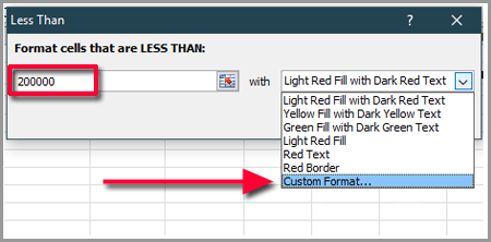
Conditional formatting with formulas (10 examples) - Exceljet You can create a formula-based conditional formatting rule in four easy steps: 1. Select the cells you want to format. 2. Create a conditional formatting rule, and select the Formula option 3. Enter a formula that returns TRUE or FALSE. 4. Set formatting options and save the rule. The ISODD function only returns TRUE for odd numbers, triggering the... Format Data Labels in Excel- Instructions - TeachUcomp, Inc. To do this, click the "Format" tab within the "Chart Tools" contextual tab in the Ribbon. Then select the data labels to format from the "Chart Elements" drop-down in the "Current Selection" button group. Then click the "Format Selection" button that appears below the drop-down menu in the same area. Excel Data Analysis - Conditional Formatting - Tutorials Point Follow the steps to conditionally format cells − Select the range to be conditionally formatted. Click Conditional Formatting in the Styles group under Home tab. Click Highlight Cells Rules from the drop-down menu. Click Greater Than and specify >750. Choose green color. Click Less Than and specify < 500. Choose red color.

Conditional formatting data labels excel. Conditional Formatting with Data Validation - Microsoft Tech Community For example, if A2=Value, B2= Value, and C2 is blank, I would like to have C2 turn red. A2,B2, and C2 all have a list range for the Data Validation. For the conditional formatting, I have only put the range to apply to as column C. The conditional formatting is not turning cells red as needed. I am not sure what the issue is. How to create a chart with conditional formatting in Excel? Add three columns right to the source data as below screenshot shown: (1) Name the first column as >90, type the formula =IF (B2>90,B2,0) in the first blank cell of this column, and then drag the AutoFill Handle to the whole column; Conditional formatting chart data labels? - Excel Help Forum The easy way to conditionally format these labels is use two series. Use something like =IF ($E2=1,0,NA ()) for the series that has red labels and =IF (#E2=1,NA (),0) for the series that has unformatted labels. Jon Peltier Register To Reply Bookmarks Digg del.icio.us StumbleUpon Google Posting Permissions Excel conditional formatting highlight row based on date 1. Select the table you will highlight rows if dates have passed, and click Home > Conditional Formatting > New Rule. See screenshot: 2. In the Edit Formatting Rule dialog box, please: (3) Click the Format button. 3. In the Format Cells dialog box, go to the Fill tab, and click to select a fill color. See screenshot:

Conditional Formatting in Excel (In Easy Steps) 1. Select the range A1:A10. 2. On the Home tab, in the Styles group, click Conditional Formatting. 3. Click Highlight Cells Rules, Greater Than. 4. Enter the value 80 and select a formatting style. 5. Click OK. Result. Excel highlights the cells that are greater than 80. 6. Change the value of cell A1 to 81. Result. How to Apply Conditional Formatting to Rows Based on ... - Excel Campus On the Home tab of the Ribbon, select the Conditional Formatting drop-down and click on Manage Rules…. That will bring up the Conditional Formatting Rules Manager window. Click on New Rule. This will open the New Formatting Rule window. Under Select a Rule Type, choose Use a formula to determine which cells to format. Excel Conditional Formatting Data Bars Select the cells that contain the data bars. On the Ribbon, click the Home tab. In the Styles group, click Conditional Formating, and then click Manage Rules. In the list of rules, click your Data Bar rule, then click the Edit Rule button. In the "Edit the Rule Description" section, the default settings are shown for Minimum and Maximum. How to Manage Conditional Formatting Rules in Microsoft Excel Go to the Home tab, click the Conditional Formatting drop-down arrow, and pick "Manage Rules.". When the Conditional Formatting Rules Manager window appears, use the drop-down box at the top to choose the sheet or to use the current selection of cells and view the rules. This allows you to jump between the rules you set up for different ...

Excel tutorial: How to add a conditional formatting key That way, we can adjust the conditions for the rules using the key itself. The first step is to create the basic layout for the key. For this, we'll set up a small table with three rows - one for each conditional format. We can then add labels for each conditional format rule. These could be anything, but let's use Excellent, Concern, and ... Custom Chart Data Labels In Excel With Formulas Follow the steps below to create the custom data labels. Select the chart label you want to change. In the formula-bar hit = (equals), select the cell reference containing your chart label's data. In this case, the first label is in cell E2. Finally, repeat for all your chart laebls. How to do conditional formatting of a label in Excel VBA Function ConditionalFormatNumber (n As Double) As String If n > 1000000 Then ConditionalFormatNumber = Format (n / 1000000, "$#,##0.00,,""M""") ElseIf n > 1000 Then ConditionalFormatNumber = Format (n / 1000, "$#,##0.00, ""K""") Else ConditionalFormatNumber = Format (n, "$#,##0.0") End If End Function Share answered Aug 24, 2017 at 9:13 Excel conditional formatting Icon Sets, Data Bars and Color Scales Select all cells in column A, except for the column header, and create a conditional formatting icon set rule by clicking Conditional Formatting > Icon sets > More Rules... In the New Formatting Rule dialog, select the following options: Click the Reverse Icon Order button to change the icons' order. Select the Icon Set Only checkbox.

Conditional Copy Data from One sheet to another workbook - Excel VBA / Macros - OzGrid Free ...

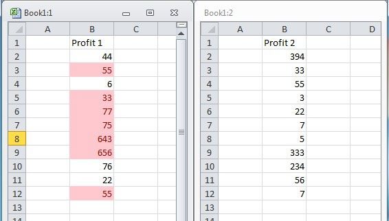
Use conditional formatting to highlight information Conditional formatting can help make patterns and trends in your data more apparent. To use it, you create rules that determine the format of cells based on their values, such as the following monthly temperature data with cell colors tied to cell values.

conditional formatting - Getting Excel to Conditionally Copy Data to Another Sheet - Super User

Conditional Formatting for a row | Microsoft Excel Tips | Excel ... Conditional Formatting For A Row In Excel You are going to learn, how to format whole row not only one cell. It can be useful for some reports or presentations. You have some sales report. You can format rows, which sales is more then 10 000$. First select your data without headings. Next go to the ribbon and click Conditional Formatting and ...

[SOLVED] Conditional copying data into another sheet

Conditional Formatting Shapes - Step by step Tutorial Let's see step by step how to create it: First, select an already formatted cell. In the picture below, we have created a little example of this. We will pay attention to the range D5:D6. You can see the rules in the Rules Manager window. We didn't make it overly complicated.

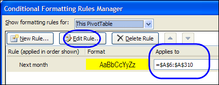
Format Pivot Table Labels Based on Date Range – Excel Pivot Tables

Creating Conditional Data Labels in Excel Charts - YouTube We can make labels appear on our charts that don't have to do with the raw numbers that built the chart - and we can make them show up or not based on whatever conditions we want. In this tutorial,...

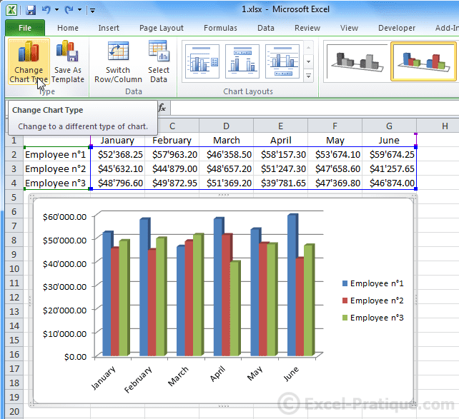
Excel Course: Inserting Graphs

How to Create Excel Charts (Column or Bar) with Conditional Formatting Conditional formatting is the practice of assigning custom formatting to Excel cells—color, font, etc.—based on the specified criteria (conditions). The feature helps in analyzing data, finding statistically significant values, and identifying patterns within a given dataset.

How to Create a MS Excel Pivot Table – An Introduction | SIMPLE TAX INDIA

Changing the Color of a Data Label using IF Statement 1) Click on the data labels to highlight all the data labels, 2) Right-Click and select Format Data Labels, 3) Click on Number, 4) Go to the Format Code field *adapt the following to your needs* 5) [green] [>29]#.00; [<30] [Color 53]#.00 Click to expand... Hi Jawnne, I hope you're still lurking about on here.

Stacked Bar Chart Data Labels Outside - Free Table Bar Chart

Conditional Formatting of Excel Charts - Peltier Tech The data for the conditionally formatted bar chart is shown below. The formatting limits are inserted into rows 1 and 2. The header formula in cell C3, which is copied into D3:G3, is =C1&"

SQL Workbench/J User's Manual SQLWorkbench

Conditional Formatting to Distinguish Between Labels and Numbers I want to conditionally format each cell, so that the text is yellow, the numbers are blue, and the blank cells are green. I tried by setting up a new rule under conditional formatting, then selecting "use a formula to determine which cells to format", then using some combinations of the if, istext, isnumber, etc. combinations. Please advise.

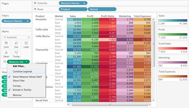
Tableau Legends Per Measure and Conditional Formatting Like Excel

Conditional formatting for Excel column charts - Think Outside The Slide Additional formatting. The colors used for each data series is from the color theme being used for this Excel file. You can assign more meaningful colors for each data series. You can also add data labels to each series. It is a good idea to format the data label text to have the same color as the column it is representing.

Excel Conditional Formatting Help - www.hardwarezone.com.sg

Change the format of data labels in a chart To get there, after adding your data labels, select the data label to format, and then click Chart Elements > Data Labels > More Options. To go to the appropriate area, click one of the four icons ( Fill & Line, Effects, Size & Properties ( Layout & Properties in Outlook or Word), or Label Options) shown here.

How to Create Multi-Category Chart in Excel - Excel Board

Excel Data Analysis - Conditional Formatting - Tutorials Point Follow the steps to conditionally format cells − Select the range to be conditionally formatted. Click Conditional Formatting in the Styles group under Home tab. Click Highlight Cells Rules from the drop-down menu. Click Greater Than and specify >750. Choose green color. Click Less Than and specify < 500. Choose red color.

Basic Conditional Formatting in Excel and Access | ExcelDemy

Format Data Labels in Excel- Instructions - TeachUcomp, Inc. To do this, click the "Format" tab within the "Chart Tools" contextual tab in the Ribbon. Then select the data labels to format from the "Chart Elements" drop-down in the "Current Selection" button group. Then click the "Format Selection" button that appears below the drop-down menu in the same area.