45 how to change excel chart data labels to custom values

support.microsoft.com › en-us › officeEdit titles or data labels in a chart - support.microsoft.com Change the position of data labels. You can change the position of a single data label by dragging it. You can also place data labels in a standard position relative to their data markers. Depending on the chart type, you can choose from a variety of positioning options. On a chart, do one of the following: Create progress bar chart in Excel - ExtendOffice 4.Then, right click the X axis, and choose Format Axis from the context menu, see screenshot:. 5.In the opened Format Axis pane, under the Axis Options tab, change the number in Maximum to 1.0, see screenshot:. 6.Then, select the performance data bar in the chart, and then click Format, in the Shape Styles group, select one theme style as you need, here, I will select …

How to Make Excel Clustered Stacked Column Chart - Data Fix A) Data in a Summary Grid - Rearrange the Excel data, then make a chart; B) Data in Detail Rows - Make a Pivot Table & Pivot Chart; C) Data in a Summary Grid - Save Time with Excel Add-In; Clustered Stacked Chart Example. In the examples shown below, there are . 2 years of data; 4 seasons of sales amounts each year; 4 different regions

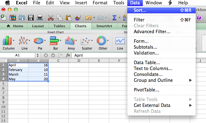
How to change excel chart data labels to custom values

Custom Data Labels with Colors and Symbols in Excel Charts - [How To] To apply custom format on data labels inside charts via custom number formatting, the data labels must be based on values. You have several options like series name, value from cells, category name. But it has to be values otherwise colors won't appear. Symbols issue is quite beyond me. Apply Custom Data Labels to Charted Points - Peltier Tech Click once on a label to select the series of labels. Click again on a label to select just that specific label. Double click on the label to highlight the text of the label, or just click once to insert the cursor into the existing text. Type the text you want to display in the label, and press the Enter key. Add or remove data labels in a chart - support.microsoft.com When the Data Label Range dialog box appears, go back to the spreadsheet and select the range for which you want the cell values to display as data labels. When you do that, the selected range will appear in the Data Label Range dialog box. Then click OK. The cell values will now display as data labels in your chart.

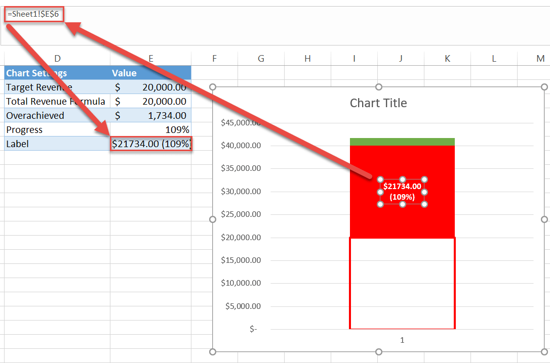
How to change excel chart data labels to custom values. Use custom formats in an Excel chart's axis and data labels Use custom formats in an Excel chart's axis and data labels . Adding a custom format to a chart's axis and data labels can quickly turn ordinary data into information. Custom Excel Chart Label Positions - My Online Training Hub Custom Excel Chart Label Positions - Setup. The source data table has an extra column for the 'Label' which calculates the maximum of the Actual and Target: The formatting of the Label series is set to 'No fill' and 'No line' making it invisible in the chart, hence the name 'ghost series': The Label Series uses the 'Value ... Excel Custom Chart Labels - My Online Training Hub Step 5: Replace the default labels with your custom labels: right-click the labels > Format Data Labels: From the 'Label Contains' list choose 'Category Name': Step 6: hide the Max series columns by formatting them with 'No fill': double-click the Max columns in the chart to open the 'Format Data Point' dialog box and under the ... Is there a way to change the order of Data Labels? Please try to double click the the part of the label value, and choose the one you want to show to change the order. Thanks, Rena ----------------------- * Beware of scammers posting fake support numbers here. * Once complete conversation about this topic, kindly Mark and Vote any replies to benefit others reading this thread. Report abuse

Excel tutorial: How to customize axis labels Here you'll see the horizontal axis labels listed on the right. Click the edit button to access the label range. It's not obvious, but you can type arbitrary labels separated with commas in this field. So I can just enter A through F. When I click OK, the chart is updated. So that's how you can use completely custom labels. Change the format of data labels in a chart - Microsoft Support To get there, after adding your data labels, select the data label to format, and then click Chart Elements > Data Labels > More Options. To go to the appropriate area, click one of the four icons ( Fill & Line, Effects, Size & Properties ( Layout & Properties in Outlook or Word), or Label Options) shown here. Add or remove data labels in a chart - support.microsoft.com Click Label Options and under Label Contains, pick the options you want. Use cell values as data labels You can use cell values as data labels for your chart. Right-click the data series or data label to display more data for, and then click Format Data Labels. Click Label Options and under Label Contains, select the Values From Cells checkbox. Change axis labels in a chart - support.microsoft.com Right-click the category labels you want to change, and click Select Data. In the Horizontal (Category) Axis Labels box, click Edit. In the Axis label range box, enter the labels you want to use, separated by commas. For example, type Quarter 1,Quarter 2,Quarter 3,Quarter 4. Change the format of text and numbers in labels

Excel charts: add title, customize chart axis, legend and data labels ... Select the chart and go to the Chart Tools tabs ( Design and Format) on the Excel ribbon. Right-click the chart element you would like to customize, and choose the corresponding item from the context menu. Use the chart customization buttons that appear in the top right corner of your Excel graph when you click on it. Improve your X Y Scatter Chart with custom data labels Press with right mouse button on on a chart dot and press with left mouse button on on "Add Data Labels" Press with right mouse button on on any dot again and press with left mouse button on "Format Data Labels" A new window appears to the right, deselect X and Y Value. Enable "Value from cells" Select cell range D3:D11 Using the CONCAT function to create custom data labels for an Excel chart Use the chart skittle (the "+" sign to the right of the chart) to select Data Labels and select More Options to display the Data Labels task pane. Check the Value From Cells checkbox and select the cells containing the custom labels, cells C5 to C16 in this example. It is important to select the entire range because the label can move based ... superuser.com › questions › 1195816Excel Chart not showing SOME X-axis labels - Super User Apr 05, 2017 · In Excel 2013, select the bar graph or line chart whose axis you're trying to fix. Right click on the chart, select "Format Chart Area..." from the pop up menu. A sidebar will appear on the right side of the screen. On the sidebar, click on "CHART OPTIONS" and select "Horizontal (Category) Axis" from the drop down menu.

10 Design Tips to Create Beautiful Excel Charts and Graphs in 2021

Present your data in a scatter chart or a line chart 09.01.2007 · As a general rule, use a line chart if your data has non-numeric x values — for numeric x values, it is usually better to use a scatter chart. Consider using a scatter chart instead of a line chart if you want to: Change the scale of the horizontal axis Because the horizontal axis of a scatter chart is a value axis, more scaling options are available. Use a …

Excel Thermometer Chart - Free Download & How to Create - Automate Excel

Change the format of data labels in a chart To get there, after adding your data labels, select the data label to format, and then click Chart Elements > Data Labels > More Options. To go to the appropriate area, click one of the four icons ( Fill & Line, Effects, Size & Properties ( Layout & Properties in Outlook or Word), or Label Options) shown here.

Mr. Krim's Class

Excel Chart Data Labels-Modifying Orientation - Microsoft Community Excel Chart Data Labels-Modifying Orientation The chart layout tab has been absorbed into other areas in Excel 2016. I cannot figure out how to change the orientation of the data labels on the axes....(tilt, horizontal, vertical).

Threshold Chart in Excel - Goodly

How to add data labels from different column in an Excel chart? Click any data label to select all data labels, and then click the specified data label to select it only in the chart. 3. Go to the formula bar, type =, select the corresponding cell in the different column, and press the Enter key. See screenshot: 4. Repeat the above 2 - 3 steps to add data labels from the different column for other data points.

Label Columns In Excel - Ythoreccio

How to Change Excel Chart Data Labels to Custom Values? First add data labels to the chart (Layout Ribbon > Data Labels) Define the new data label values in a bunch of cells, like this: Now, click on any data label. This will select "all" data labels. Now click once again. At this point excel will select only one data label.

Excel Vba Chart Horizontal Axis Labels - vba excel charts enter array as xvalue on date axis ...

Multiple Time Series in an Excel Chart - Peltier Tech 12.08.2016 · Here is the data for our dummy series, with X values for the first of each month and Y values of zero so it rests on the bottom of the chart. Hide the axis labels by using a custom number format of ” ” (a space surrounded by quotes). If we just set the axis to show no labels, the margin below the axis would have collapsed, but using this dummy number format uses a …

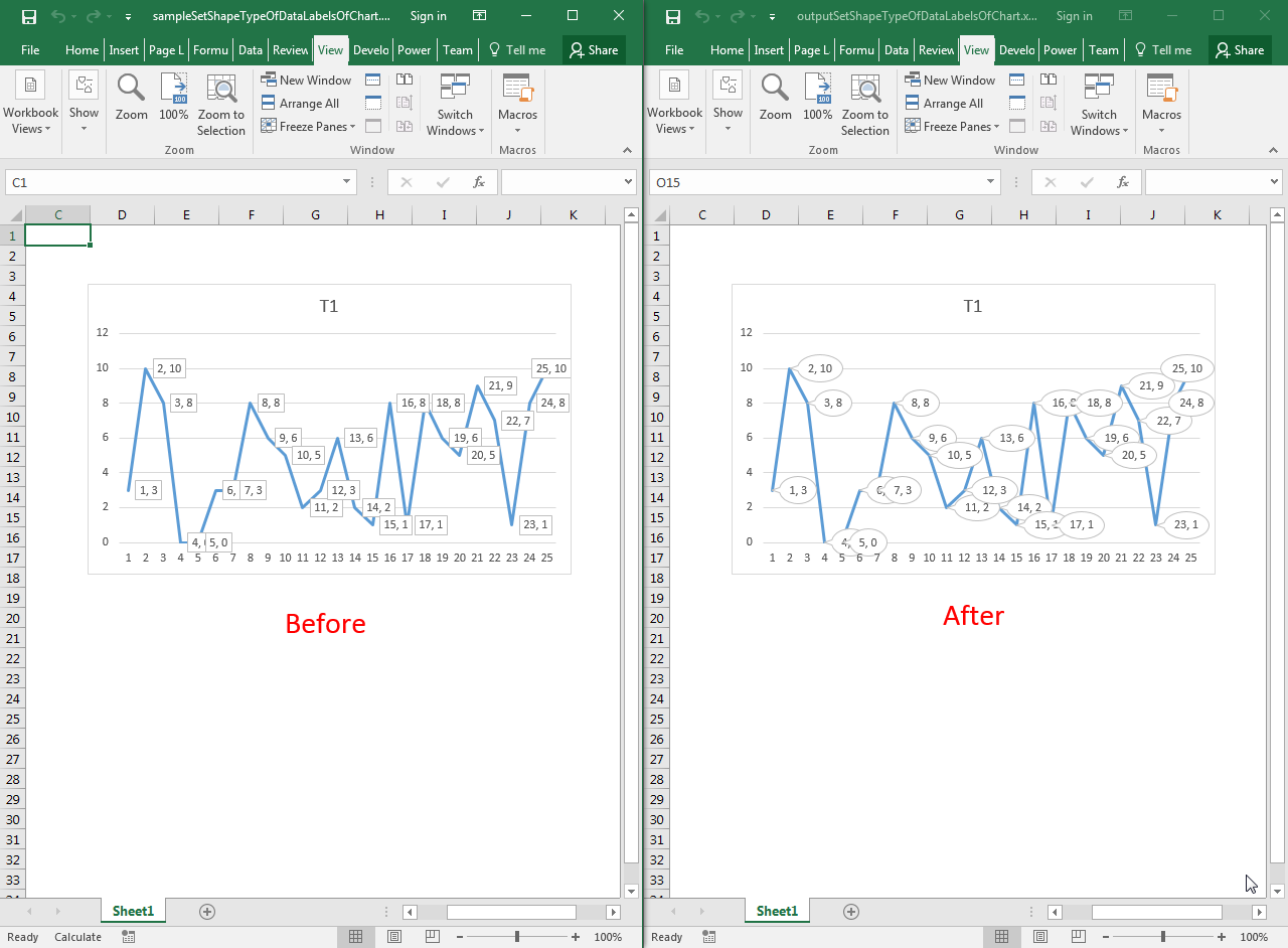
Set the Shape Type of Data Labels of Chart | Documentation

How to create Custom Data Labels in Excel Charts Two ways to do it. Click on the Plus sign next to the chart and choose the Data Labels option. We do NOT want the data to be shown. To customize it, click on the arrow next to Data Labels and choose More Options … Unselect the Value option and select the Value from Cells option. Choose the third column (without the heading) as the range.

30 How To Label A Column In Excel - Labels Design Ideas 2020

How to add and customize chart data labels - Get Digital Help The image above demonstrates data labels in a line chart, each data point in the chart series has a visible data label. Edit data labels. Excel allows you to edit the data label value manually, simply press with left mouse button on a data label until it is selected. Press with left mouse button on again to select the text, you can now type any ...

Share :