42 excel pivot table labels

Excel: How to Filter Data in Pivot Table Using "Greater Than" To do so, click the dropdown arrow next to Row Labels, then click Value Filters, then click Greater Than: In the window that appears, type 10 in the blank space and then click OK: The pivot table will automatically be filtered to only show rows where the Sum of Sales is greater than 10: To remove the filter, simply click the dropdown arrow next ... › Create-Pivot-Tables-in-ExcelHow to Create Pivot Tables in Excel (with Pictures) - wikiHow May 05, 2021 · A Pivot Table allows you to create visual reports of the data from a spreadsheet. You can perform calculations without having to input any formulas or copy any cells. You will need a spreadsheet with several entries in order to create a Pivot Table. You can also create a Pivot Table in Excel using an outside data source, such as Access. You can ...

› xlpivot08Excel Pivot Table Multiple Consolidation Ranges Create a Pivot Table from Multiple Sheets. To see how to create a pivot table from data on different sheets, watch this short video. The written instructions are below. Note: To see the video transcript, go to the Multiple Sheets Video page. Introduction. Create the pivot table. Clean up the pivot table

Excel pivot table labels

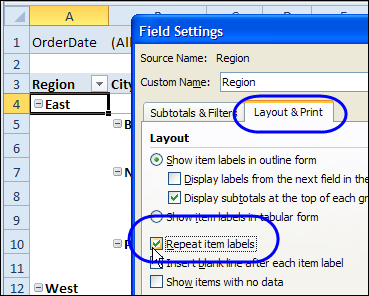
Repeat Pivot Table row labels - AuditExcel.co.za So to repeat pivot table row labels, you can right click in the column where you want the row labels repeated and click on Field Settings as shown below. In the Field Settings box you need to click on the Layout & Print tab and choose the 'Repeat items labels'. Like magic you will now see the row labels repeated on every line. Filter by Labels - Text | MyExcelOnline STEP 1: Click on the Row Label filter button in the Pivot Table. STEP 2: Select Label Filters. You will see that we have a lot of filtering options. Let us try out - Ends With. STEP 3: Type in ber to get the months ending in ber. You can see that the Label Filter will be applied to the SALES MONTH. Click OK. Pivot Table in Excel - A Beginners Guide for Excel Users Row labels: One or more rows in the pivot table can be filtered using row labels. Values 'Values' takes a field that has numerical values in it, which can be used for different types of calculations. Column field: Column fields are the ones which has a column orientation in the pivot table. Each item in the field occupies a column and it ...

Excel pivot table labels. powerspreadsheets.com › excel-pivot-table-groupExcel Pivot Table Group: Step-By-Step Tutorial To Group Or ... Let's start by looking at the… Example Pivot Table And Source Data. This Pivot Tutorial is accompanied by an Excel workbook example. If you want to follow each step of the way and see the results of the processes I explain below, you can get immediate free access to this workbook by subscribing to the Power Spreadsheets Newsletter. Excel 2021 (Mac) - pivot tables - "Show items labels in tabular form" Just purchased Office 2021 (Mac) - on the PC version for pivot tables - in the "Field Settings", under the "Layout & Print" tab, there is a "Show items labels in tabular form" - is this function available in the Mac version - I cannot find it? If not is there anyway to accomplish the same via a different method on the Mac version Labels: PivotTable.RepeatAllLabels method (Excel) | Microsoft Docs Return value. Nothing. Remarks. Using the RepeatAllLabels method corresponds to the Repeat All Item Labels and Do Not Repeat Item Labels commands on the Report Layout drop-down list of the PivotTable Tools Design tab.. To specify whether to repeat item labels for a single PivotField, use the RepeatLabels property.. Support and feedback. Have questions or feedback about Office VBA or this ... Pivot table field list hard to read - white text on light grey ... Hi, I've had a problem with the field list in the pivot table being hard to read. All of the sudden it started showing up as white text on a light grey background. Just in teh filters, columns, rows and values windows. ... Excel Charting & Pivots [SOLVED] Pivot table field list hard to read - white text on light grey background; Results 1 to 3 of 3

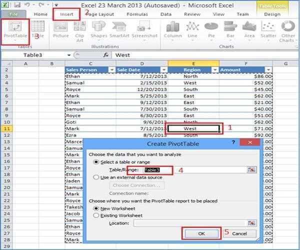
How to Create a Pivot Table in Microsoft Excel Excel then reviews your data for tables that fit. Go to the Insert tab and click "Recommended PivotTables" on the left side of the ribbon. When the window opens, you'll see several pivot tables on the left. Select one to see a preview on the right. If you see one you want to use, choose it and click "OK.". How to Create Excel Pivot Table [Includes practice file] To create an Excel pivot table, Open your original spreadsheet and remove any blank rows or columns. You may also use the Excel sample data at the bottom of this tutorial. Make sure each column has a meaningful label. The column labels will be carried over to the Field List. Verify your columns are properly formatted for their data type. How To Create A Pivot Table In Excel - Naukri Learning Step 1 - Insert your data on the excel sheet. Click any cell in the source data and go to the Insert tab. Click the PivotTable button inside the Tables group. You can also choose the Recommended PivotTables option to check for other options. Excel offers other previews to insert your dynamic periodic table. Copy Pivot Chart messes up Data Labels - Microsoft Community I am trying to copy a Pivot Chart and paste it into Power Point. What happens is that Data-Labels that have been deleted in the excel (like 0%) reappear when pasting. This happens regardless of copied as object or picture/ pasted as object or picture. The funny thing is: When I paste in PowerPoint as object, THEN delete the labels, then copy ...

excel-Pivot Table Label Filter Is Applied But Data Does Not Actually ... Clicking on this header icon shows that a label filter has been applied and when I click to the filter itself: Filter in header --> Label Filters --> Not Between .....I see the -10 and 10 in the value fields. The issue is that the actual data in the pivot table does not reflect the filter - it has not been applied (ie. stackoverflow.com › questions › 50336509Combining Column Values in an Excel Pivot Table - Stack Overflow May 14, 2018 · In your pivot table, Select the Pivot Table Tools> Analyze tab, then "Fields, Items",then pull down to"Calculated fields". Enter a name for the generated field, and the formula you want to use: In my example, I added the fields Fruit and Vegi's from my available pivot table fields (which is based on my data table). › blog › insert-blank-rows-inHow to Insert a Blank Row in Excel Pivot Table | MyExcelOnline Jan 17, 2021 · Pivot Table reports are shown in a Compact Layout format as a default and if you have two or more Items in the Row Labels (e.g.Month & Customer), then the Pivot Table report can look very clunky… There is a cool little trick that most Excel users do not know about that adds a blank row after each item, making the Pivot Table report look more ... Exclude (blank) from PivotTable row label | MrExcel Message Board Use the new column in your pivot instead of the current column. The apply the label filter for not equal to [No Name] or whatever you end up using. Donors was my table name it will change when you select the UUK Name field. Excel Formula: =if(Donors[UUK Name]=""," [No Name]",Donors[[UUK Name]) Dealing with Blanks in Your Data Model FrankieGTH F

How to Increase Indent Row Labels in Pivot Table Compact Form - ExcelNotes

Show/Hide Field Headers in Excel Pivot Tables | MyExcelOnline Whenever you work with Pivot Tables, you can see the Row Labels and Column Labels that are automatically generated on top. This is handy as they can be used to filter out your records. But, Pivot Table being a tool for the presentation of data as well, you might want to hide these labels as well for making the data set more presentable.

Add label to Excel chart line • AuditExcel.co.za

Pivot Tables in Excel - Excel IF | No 1 Excel tutorial on the net Insert a Pivot Table To insert a pivot table, execute the following steps. 1. Click any single cell inside the data set. 2. On the Insert tab, in the Tables group, click PivotTable. The following dialog box appears. Excel automatically selects the data for you. The default location for a new pivot table is New Worksheet. 3. Click OK. Drag fields

How to Sort Data in a Pivot Table | Excelchat

How to Filter Excel Pivot Table (8 Effective Ways) - ExcelDemy ⏩ Click on the drop-down arrow of Row Labels. ⏩ Go to Value Filters > Top 10. ⏩ Input 5 instead of 10 and press OK. This is the expected output. 2.2. Value Filters to Return Say, you want to filter the top 50% sum of sales from the total sum of sales. For finding out this, just go on the Top 10 Filter option likewise the previous example.

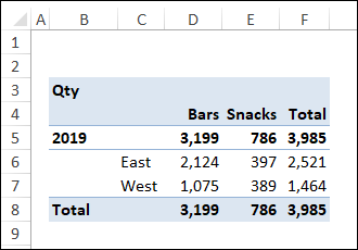
Microsoft Excel Pivot table repeat item labels - HowToAnalyst

› excelpivottablemovelabelsHow to Move Excel Pivot Table Labels Quick Tricks To move a pivot table label to a different position in the list, you can use commands in the right-click menu: Right-click on the label that you want to move Click the Move command Click one of the Move subcommands, such as Move [item name] Up The existing labels shift down, and the moved label takes its new position. Type Over Another Label

MS Excel 2011 for Mac: Display the fields in the Values Section in multiple columns in a pivot table

Excel Pivot Table tutorial - Ablebits When you are creating a pivot table, Excel applies the Compact layout by default. This layout displays " Row Labels " and " Column Labels " as the table headings. Agree, these aren't very meaningful headings, especially for novices. An easy way to get rid of these ridiculous headings is to switch from the Compact layout to Outline or Tabular.

15 Pivot Table ideas | pivot table, excel, excel tutorials

Advanced pivot table features in Numbers on iPhone, iPad, and Mac Learn more about pivot table snapshots and how to create them in Numbers on Mac, in Numbers on iPhone, and in Numbers on iPad . Editable labels To edit labels in a pivot table, create a snapshot of the pivot table, then edit labels in the snapshot of the pivot table. Manually organized rows and columns

Pivot Table Excel 2007 Repeat Row Labels | Elcho Table

PivotField.LabelRange property (Excel) | Microsoft Docs In this article. Returns a Range object that represents the cell (or cells) that contain the field label. Read-only. Syntax. expression.LabelRange. expression A variable that represents a PivotField object.. Example. This example selects the field button for the field named ORDER_DATE.

Excel - Pivot Table - Custom, show group by labels in tabular form for sum, count, etc. - YouTube

Excel filtering pivot table filter/slicer across column label Excel filtering pivot table filter/slicer across column label. Hello. I have a table with the year as the column headings/labels (2009-2021) and a couple other columns with additional information that aren't a year. The rows represent the specific data for each year. I have made a pivot table and slicers for the columns with the other date but ...

Hide Excel Pivot Table Buttons and Labels – Excel Pivot Tables

How to sort columns in pivot table in Excel | Basic Excel Tutorial Having created the PivotTable, the first step in sorting column data. We click the field with the data or items that need Sort. The option is at the Pivot table. Click Sort on the data tab, then choose the type of order you wish to sort your data. If your option is not on the displayed options, additional options are available on the Click Options.

How to group (two-level) axis labels in a chart in Excel?

How to Use Excel Pivot Table Label Filters In an Excel pivot table, you might want to hide one or more of the items in a Row field or Column field. To do that, you could click the drop down arrow for the Row or Column Labels, then remove the check mark for items you want to remove. For example, to hide the data for 7-Feb-10, you'd click on the check mark to remove it.

Excel Pivot Table Report - Sort Data in Row & Column Labels & in Values Area, use Custom Lists

Pivot Table "Row Labels" Header Frustration - Microsoft Tech Community Small and Medium Business. Public Sector. Internet of Things (IoT) Azure Partner Community. Expand your Azure partner-to-partner network. Microsoft Tech Talks. Bringing IT Pros together through In-Person & Virtual events. MVP Award Program. Find out more about the Microsoft MVP Award Program.

Excel Pivot Table Report - Sort Data in Row & Column Labels & in Values Area, use Custom Lists

Excel Pivot values as column labels - Stack Overflow If you have Excel for Office 365 (or Excel 2021) with the FILTER function, you can use the following: Note that I used a table with structured references for the data source. This has advantages in editing the table in the future. For "pivot" header: =TRANSPOSE(SORT(UNIQUE(Table1[Country]))) For the columns:

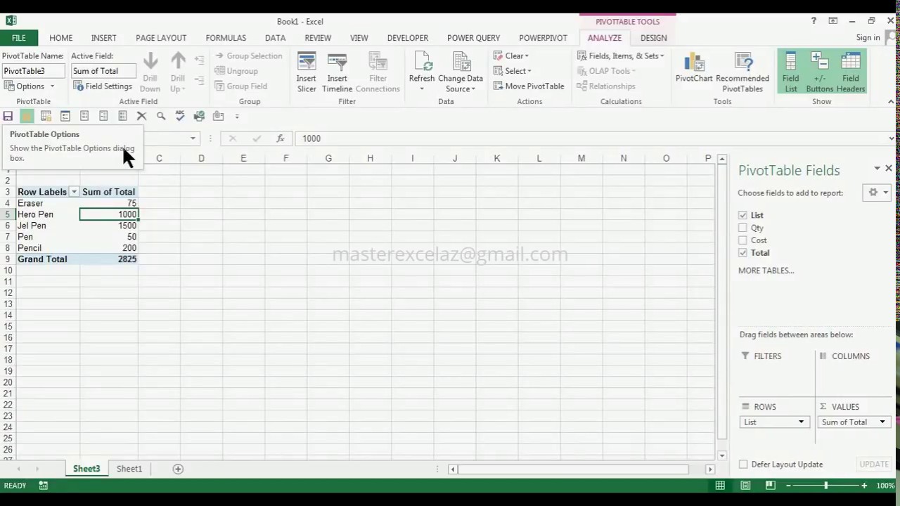
How to get Pivot Table Tools Analyze Tab in MS Excel 2013 | Basic excel skill - YouTube

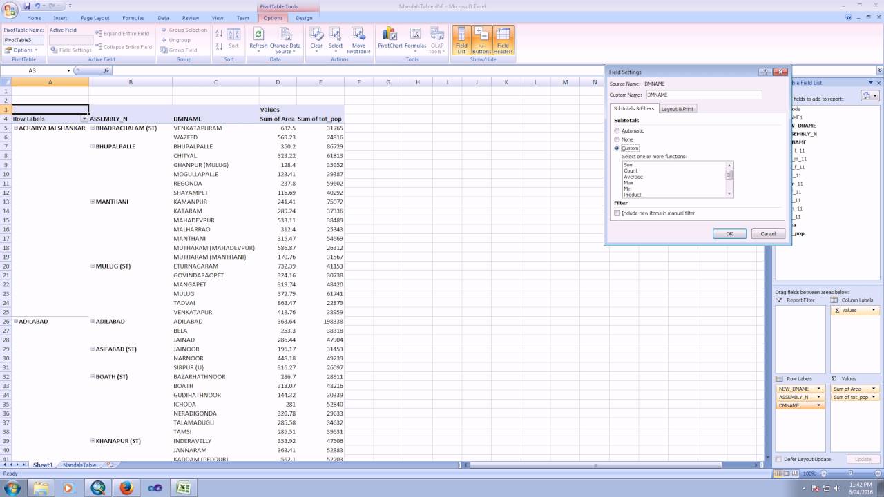
Repeat first layer column headers in Excel Pivot Table Right-click the row or column label you want to repeat, and click Field Settings. Click the Layout & Print tab, and check the Repeat item labels box. Make sure Show item labels in tabular form is selected. Tested just now and it worked for column headers. Thanks for the link, Alan.

Repeat Pivot Table Labels in Excel 2010 - Excel Pivot TablesExcel Pivot Tables

Excel: How to Sort Pivot Table by Date - Statology Often you may want to sort the rows in a pivot table in Excel by date. Fortunately this is easy to do using the sorting options in the dropdown menu within the Row Labels column of a pivot table. The following example shows exactly how to do so. Example: Sort Pivot Table by Date in Excel

Pivot Table in Excel

3 Tips for the Pivot Table Fields List in Excel - Excel Campus Pivot Table Fields List Tips.xlsx. The Pivot Table Task Pane. When working with pivot tables, there's is a task pane that is used to add or delete fields to different areas of the table. This is the Pivot Table Fields list and I'd like to share with you three tips to help you use it more efficiently. Tip #1: Change the Layout of the Field List

Use excel pivot table layout to add label to entry - Stack Overflow

trumpexcel.com › group-numbers-in-pivot-tableHow to Group Numbers in Pivot Table in Excel Sometimes, numbers are stored as text in Excel. In such case, you need to convert these text to numbers before grouping it in Pivot Table. You May Also Like the Following Pivot Table Tutorials: How to Group Dates in Pivot Table in Excel. How to Create a Pivot Table in Excel. Preparing Source Data For Pivot Table. How to Refresh Pivot Table in ...

Grouping in Excel Pivot Tables - YouTube

How to Create a Pivot Table in Excel: A Step-by-Step Tutorial Highlight your cells to create your pivot table. Drag and drop a field into the "Row Labels" area. Drag and drop a field into the "Values" area. Fine-tune your calculations. Now that you have a better sense of what pivot tables can be used for, let's get into the nitty-gritty of how to actually create one. Step 1.

Share :